Sometime with repeated measures data is it useful to look at the trend in the data - something that can be achieved with polynomial contrasts.
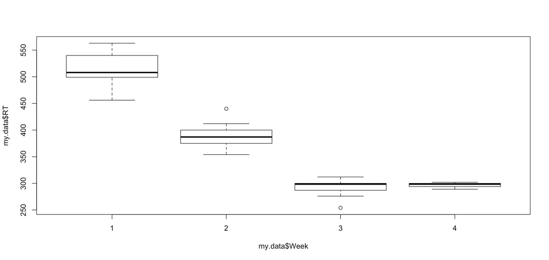
Load the data HERE into a table and plot it using the following commands:
my.data = read.table('sampleRMData.txt')
names(my.data) = c('Subject','Week','RT')
my.data$Subject = factor(my.data$Subject)
my.data$Week = factor(my.data$Week)
plot(my.data$RT~my.data$Week)
Load the data HERE into a table and plot it using the following commands:
my.data = read.table('sampleRMData.txt')
names(my.data) = c('Subject','Week','RT')
my.data$Subject = factor(my.data$Subject)
my.data$Week = factor(my.data$Week)
plot(my.data$RT~my.data$Week)
So, imagine this is performance data and you want to show a trend in the data - for example a quadratic trend to relate this to the Power Law of Practice. You can do that easily with the emmeans package and polynomial contrasts.
Try the following code:
install.packages('emmeans')
library('emmeans')
myRMANOVA = aov(RT ~ Week + Error(Subject / Week), data = my.data)
print(summary(myRMANOVA))
weekContrast = emmeans(myRMANOVA,"Week")
poly = contrast(weekContrast,'poly')
print(poly)
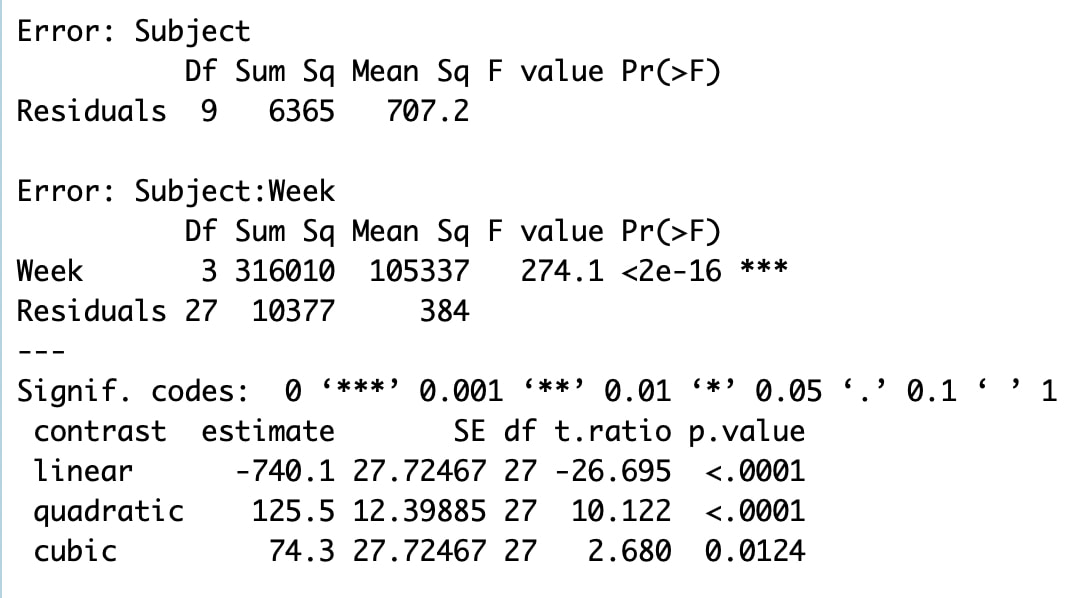
You should see the following output:
Try the following code:
install.packages('emmeans')
library('emmeans')
myRMANOVA = aov(RT ~ Week + Error(Subject / Week), data = my.data)
print(summary(myRMANOVA))
weekContrast = emmeans(myRMANOVA,"Week")
poly = contrast(weekContrast,'poly')
print(poly)
You should see the following output:
So, you have a significant repeated measures ANOVA, given the data, not surprising. However, you also have significant linear and quadratic trends! You could report these to argue practice effects as opposed to reporting the results of paired sample t-tests.

