In this assignment you will learn to do a repeated measures ANOVA.
First, load the data HERE into a data frame called data. This is actually the same data as for Assignment 7B but there is one important change. You will note that the participant numbers repeat themselves from 1 to 50 three times. This makes complete sense, as in a repeated measures ANOVA you have the same participants doing the same thing on repeated measurements (i.e., measurements over time) or you have the same participants completing a series of experimental conditions. Examining the participant numbers is an easy way to tell if long format data is for a between or within design. Indeed, in order to run a repeated measures ANOVA in R it is crucial that the participant numbers be accurate. If you are used to repeated measures ANOVA in SPSS you will note that in R long format is used for both between and within designs whereas in SPSS repeated measures ANOVA data is typically in a wide or column format.
Running a RM ANOVA is easy to do in R.
data = read.table("samplermanovadata.txt")
names(data) = c("subject","condition","data")
data$subject = factor(data$subject)
data$condition = factor(data$condition)
model = aov(data$data~data$condition+Error(data$subject/data$condition))
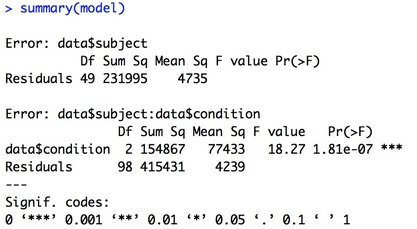
summary(model)
You will note one key difference in the aov command, and that is the Error term. If you recall the theory behind RM ANOVA, you are removing between participant variance from the overall error variance. This error term accomplishes just that.
Testing Assumptions
Here I will only review how to test the assumption of sphericity as you can easily refer to Assignment 7A for how you would test the assumptions of normality and homogeneity of variance.
The Assumption of Sphericity: The assumption of sphericity is that the variances of the difference scores are equal.
The reality is that in R the test of this assumption is not as easy as one might think. Indeed, it is easier to just run the RM ANOVA using the ezANOVA package.
install.packages("ez")
library("ez")
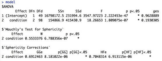
model = ezANOVA(data=data, dv = .(data), wid =.(subject), within =.(condition), detailed = TRUE, type = 3)
model
This will give you a full RM ANOVA table plus the test of sphericity. Note, if you fail the test of sphericity you should use one of the corrected p-values and correct the degrees of freedom. In general, the closer epsilon is to 1 then the more closely the assumption is met. The lower bound of epsilon is defined as 1/(number of levels - 1). So, for this design epsilon should have a range between 0.5 and 1. If epsilon is closer to the lower bound than 1 then the assumption is definitely not met. Things you can do if the assumption of sphericity is not met:
1. Use the Greenhouse-Geisser Correction
i. Use the new p value
ii. Correct the degrees of freedom by multiplying by epsilon
2. Use the Huynh-Feldt Correction (better to use this for E > 0.75 or n is small, less than 15)
i. Use the new p value
ii. Correct the degrees of freedom by multiplying by epsilon
3. Use an average of the two epislon values and p values.
Post-Hoc Analysis of RM ANOVA
To post-hoc this data all you need to do is run a series of pairwise comparisons:
pairwise.t.test(data$data,data$condition,paired=TRUE)
Another option would be to conduct a trend analysis, this will be described in full in assignment 7D.
Assignment 7C
For the data HERE, run a complete repeated measures analysis. Test all of the assumptions, run the ANOVA, and complete a pairwise post-hoc analysis

