In this assignment you will learn how to do a multiple regression. Note, MR is a very complicated topic - the point of this tutorial is simply to show you how to do multiple regression in R. For understanding of the material, I strongly recommend you read Chapter 6 and 7 the Field textbook.
1. Load the data file HERE into a variable called data.
2. For simplicities sake, let's make the following variable assignments:
y = data$V1
x1 = data$V2
x2 = data$V3
x3 = data$V4
x4 = data$V5
x5 = data$V6
x6 = data$V7
This is simply just assigning the variables in the data frame columns to separate variables.
3. Running a multiple regression in R is easy. If you wanted to see how the variables x1, x2, x3, x4, x5, and x6 predicted y you would simply write:
results = lm(y~x1+x2+x3+x4+x5+x6)
summary(results)
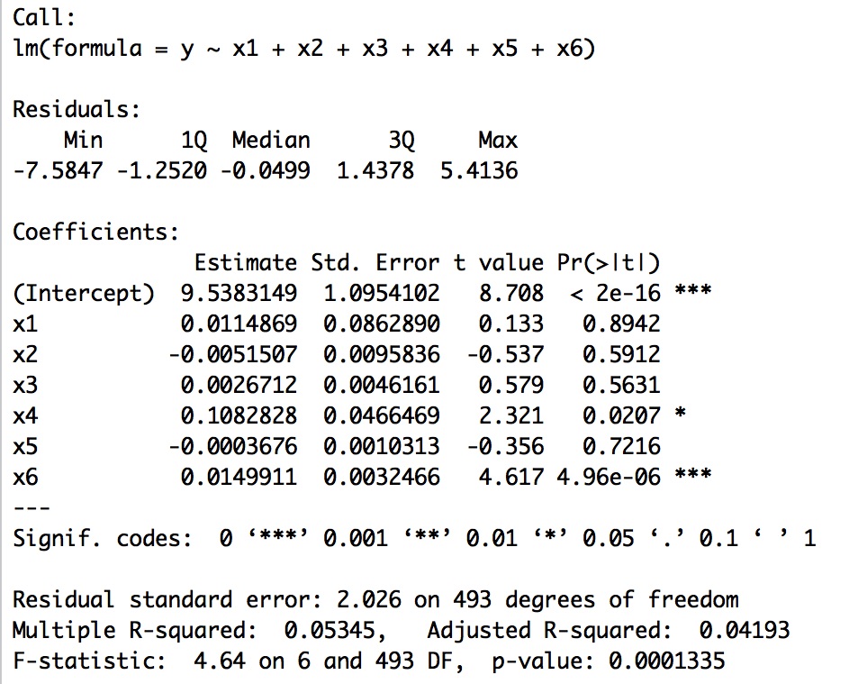
You should see something that looks like this:
|
At the top you see the call - you are telling R to create a linear model where y is a function of x1, x2, x3, x4, x5, and x6.
You then get the residuals of the model. What are residuals? The residuals are the differences between the predicted and actual y values. What R is showing you here is information about the residuals as a whole - the minimum and maximum values, the values of the 1st and 3rd quartiles, and the median. R next provides you with the regression coefficients, the standard error for each coefficient, and the significance test of each coefficient. In this case, you will note that variables x4 and x6 significantly contribute to the model. We will do more on model evaluation and comparison later, but the short version is only x4 and x6 are needed to accurately predict y (sort of). Finally, R provides you with an overall test of the model (is there a linear model that fits the data?) and the R-squared value (actual and adjusted) - in other words, the proportion of variance in the data explained by the model. |
Testing the Assumptions of Multiple Regression
Statistical assumptions are the criteria that must be met for a statistical test to be valid. In other words, if you do not meet these criteria then the results of the test may be invalid.
1. The Assumption of Independence of Errors
When you use multiple regression it is important to test whether or not there is an independance of the errors (residuals) in the model - another term for this is to check the autocorrelation of the errors. In R, this is easy to do using a Durbin Watson Test. However, this test is in the car package so:
install.packages("car")
library(car)
durbinWatsonTest(results)
You should see that D-W statistic is 1.996064 which is good (you want this value to be between 1 and 3 and as close to 2 as possible). You will also see that the result of this test is non-significant which is also good.
2. The Assumption of Multicollinearity
In general, you do not want variables in a multiple regression to be highly correlated - when they are this is collinearity. To test this, we typically examine VIF or variance inflation factors. In R, it is easy to generate a few statistics to check the multicollinearity of the data. The three criteria are:
i. No VIF above 10 - check with vif(results).
ii. The average VIF should be close to 1- check with mean(vif(results))
iii. Ideally, the tolerance (1/vif) should be not be less than 0.1, and less than 0.2 may be a problem - check with 1/vif(results)
3. The Assumption of Normality, Linearity, and Homoscedasticity of Residuals
While this is not one of the actual assumptions of multiple regression, one simple test of the assumptions in R is to examine the residuals. If the residuals are normally distributed then one can generally assume that all of the assumptions have been met.
res = resid(results)
This command puts all of the residuals (the difference between the actual and predicted y values) into a variable called res.
hist(res)
If the histogram is normally distributed, then one can assume the assumptions were met. One could also formally test the distribution with a statistical test if desired to gauge normality. It is also worth noting that if the histogram looks normal it suggests there are no outliers in the data (but this may be wrong, see below).
Using Q-Q Plots to Examine Normality
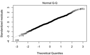
Another thing to check is the Q-Q plot of the data. The Q-Q plot in a multiple regression shows deviations from normality thus you want it to be straight. You can see the multiple regression plots by using:
plot(results)
Hit RETURN until you see the Q-Q plot, which in this case, looks just fine.
4. The Absence of Outliers and Influential Cases
As with any analysis, outliers and certain data points can push the analysis around quite a bit. A simple way to examine for multivariate outliers is to compute either a Cook's Distance or Malhabanonis Distance from the multivariate centroid of the data. In R, this is easy to do:
cooks = cooks.distance(results)
plot(cooks)
You will note quite clearly on the plot that there is an outlying value that should be removed from the data and the WHOLE analysis should be rerun with this data point removed.
Assignment 6C
1. Load the data HERE.
2. Assume the data in the first column is the predicted variable and the other columns are predictor variables. Run a multiple regression in R. Which variables contribute to the model? Which do not? BONUS. Run a model comparison in R between a reduced model including only the significant predictor variables and the full model to show they are the same. There is a bit on this in the Field textbook.
3. Test each of the four assumptions outlined above.


