2A. The Mean, Median, and Mode

1. Okay, load the same data you used in Exercise 2. Label the columns the same way they were labelled for that exercise as well.
2. One of the most important descriptive statistics is the MEAN, or AVERAGE. The MEAN is just a number that represents the average of arithmetic MEAN of the data. But think about what a MEAN really is – it is a descriptor of performance. If a baseball player has a mean batting percentage of 0.321 it means they contact the ball on average 32.1% of the time. In other words, that is there average performance. If the player starts hitting more consistently, the mean goes up. Why? Because you have added a series of scores that push that are greater than the previous mean – thus the average score goes up. The reverse is also true if the player starts missing. Never lose sight of the fact that the mean reflects a series of scores and that changes in those scores over time change the mean.
3. In R, to calculate the mean simply use: mean(mydata$rt)
Before we move on, it is important that you understand what a mean really is. Of course, it is an average, but what does that mean? (no pun intended!)
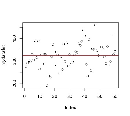
Look at the following plot of mydata$rt. (Note, you can do this yourself by using plot(mydata$rt)
I have also used abline(a = mean(mydata$rt), b = 0, col = "red") to add a red line representing the mean. If you look at the command it specifies a y intercept a which is equal to the mean, a slope b = 0 and makes the line colour red.
Now, what is the mean? Yes, it is an average of your the numbers in mydata$rt. BUT, it is also a model for your data. What do we mean by model? The mean value (325.661) represents the data - it is the model of this data. Think of it this way - if you were going to predict the next number in the series of numbers mydata$rt, what number would you pick? The best guess would be the mean as it is the average number. So, the mean is a model of the data. You can read more about this notion HERE and HERE.
Okay, now load in a new data file, data2.txt which is HERE, into a data table called income (see the bottom of this page for HINTS if you cannot remember or figure out how to do this). This file contains 10000 data points, each of which represents the income of a person in a Central American country in US dollars. NOTE, R check to see what the column label is in the new data table. It may not be V1, etc.
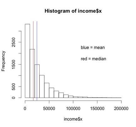
Here is a histogram of income. You can generate this yourself easily by using the command hist, e.g., hist(income$x).

Note the shape of the data. We will data about distributions of data later, but this is what is called a skewed distribution.
Determine the mean and median of the income$x. HINT, mean(income$x) and median(income$x).
You should find that the mean is 24654.92 and the median is 17203.5.
First, you should review a full definition of a median, but it is essentially the score at the 50th percentile, or the middle of a distribution of numbers. A good definition of the median is HERE.
In terms of the data set income$x, which is a better model for the data, the mean or the median? Think of it this way, if you moved to the country that you this data is from, would you expect your income to be closer to 17203 or 24654? The correct answer in this case is 17203 given the distribution of the data. This is important to realize. A lot of time in statistics we become obsessed with using the mean as a model of our data. However, sometimes the median is a better model for your data - especially in cases like this where it is heavily skewed. Note, for normal data the mean and median should be very similar. Compare the mean and median for mydata$rt. You should see that they are very close, differing by 2 points, 325.661 versus 327.7983.
I am not going to say much about the mode. Although the mode is frequently mentioned in statistics textbooks, I can honestly say in my 15 years as a researcher I have never computed a mode other than when I teach statistics.
Logical Indexing
One of the reasons R is so powerful for statistics is that is supports logical indexing. What I mean by that, is that in our data set mydata$rt I have included codes (mydata$group) to highlight that the reaction time data is from two groups of participants. So, if you type in mean(mydata$rt) you get the mean across both groups of participants. However, if you wanted to simply get the mean of the mydata$rt for participants in group one you would type mean(mydata$rt[mydata$group==1]). R will interpret this to give you the mean for mydata$rt only for cases where the variable mydata$group is 1.
4. Your assignment for the week - compute the mean and median for groups 1 and 2 separately for both variables, mydata$rt and mydata$eeg. Use the plot command and the abline function to plot the mean and median for both variables as per the first plot on this page. Plot the mean in red and the median in blue.
HINTS
income = read.table("data2.txt")
income = read.table("data2.txt")