ANOVA
In earlier lessons you learned how to test to see whether or not two groups differed - an independent samples t-test. But what do you do if you have more than two groups?
The first case we will examine is when you have three or more independent groups and you want to see whether or not there are differences between them - the test that accomplishes this is an Analysis of Variance - a between subjects test to determine if there is a difference between three or more groups.
Analysis of Variance (ANOVA) is a complex business, at this point you need to find a textbook and read the chapter(s) on ANOVA. For a quick summary you can go HERE, but that is not really going to be enough.
Load this DATA into a new table called "data" in R Studio. You will note the first column indicates subject numbers from 1 to 150, the second column groups codes for 3 groups, and the third column actual data. Rename the columns "subject", "group", and "rt".
Lets define group as a factor. Remember how to do that?
data$group = factor(data$group)
Of course you can use graphics to get a feel for what is happening. Let's try a boxplot:
boxplot(data$rt~data$group)
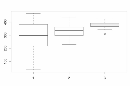
Box plots show differences between factors (each group) but they also provide information about the data within each group. The boxes represent the data that falls between the 25th and 75th percentile, the bottom and top of the error bars show the range from the 1st to 100th percentile, the line in the middle of the box reflects the median, and any circles that appear are suggested outliers.
However, the point of an ANOVA is to statistically assess whether or not there are differences between the three groups. As it turns out, this is very easy to do:
analysis = aov(data$rt~data$group)
This command tells R to run an analysis of variance (aov) on data$rt with data$group as a factor. To see the actual results of the ANOVA, you need to type: summary(analysis). What you will see is the ANOVA summary table.
analysis = aov(data$rt~data$group)
This command tells R to run an analysis of variance (aov) on data$rt with data$group as a factor. To see the actual results of the ANOVA, you need to type: summary(analysis). What you will see is the ANOVA summary table.
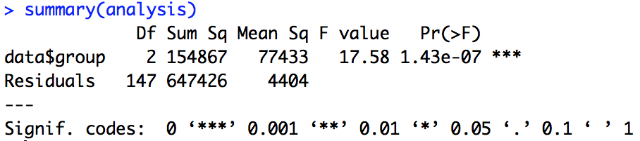
The summary table gives you a lot of key information. Perhaps the most important are the F statistic and the p-value - in this case the p value is below 0.05 so the ANOVA suggests that there are differences between the groups.
Note, typically you would report this ANOVA as follows. Our analysis revealed that there was a difference between groups, F(2,147) = 17.58, p < 0.001.
There is something important to note here - an ANOVA simply tells you whether or not there is a difference between groups, it does not tell you where the difference is. See below and Lesson 7C.
The box plot above suggested this, another way to show this would be to plot the means with error bars. To do this, we need to add the library "gplots". See Lesson 1A but you can do the following:
install.packages("gplots")
library("gplots")
If you recall, this will install the gplots library and then the library command will load it. Now, to plot the group means with 95% confidence intervals as the error bars you can simply use:
plotmeans(data$rt~data$group)
For more understanding...
The short version is that ANOVA is a special case of multiple regression - it is just a form of a linear model.
Try the following:
model1 = aov(data$rt~data$group)
summary(model1)
Look at the F statistic and p-value.
model2 = lm(data$rt~data$group)
summary(model2)
Look at the t statistics and p-value (recall F = t^2!!!). They are the same but the data is represented in a regression format because it was defined as a linear model and not a special case. To recover the ANOVA table.
anova(model2)
Assignment Question
The data HERE reflects data from 4 groups of people, with each group reflecting data from a different city. Run the ANOVA. What is the story here? What cities are the same and what cities differ? Ensure you report the results of your ANOVA and support your claims of group differences and similarities with a plot and with the results of a TukeyHSD test. Ensure that you make a statement and test all of the assumptions of ANOVA (see Lesson 7A).